International Journal of Mechanical Engineering and Mechatronics (IJMEM)

ISSN: 1929-2724

1. Introduction

"The wall jet is a type of shear layer flow along a wall that due to its initial momentum, at any station, its streamwise velocity in some point is higher than the velocity of the external flow" [1]. Boundary layer control in advanced aircrafts, film cooling of combustion chambers and turbine blades, and air conditioning systems are typical examples for engineering applications of wall jets.  The schematic of the velocity distribution in a two-dimensional wall jet with a slot height of b and jet discharge velocity of U_j is shown in Figure 1. 

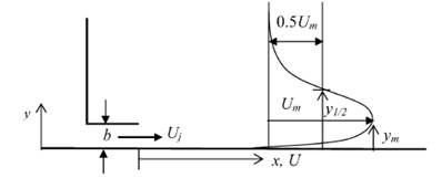
The velocity profile shows a maximum axial velocity, U_m, which occurs at height of y_m (see Figure 1). There are two different shear flows in the wall jet. The first one which starts from the wall and extends to the point of maximum velocity has typical characteristics of a boundary layer and traditionally is called the inner region. The second shear flow starts from the point of maximum velocity and extends to the other edge of the flow. It is called the outer region and has the characteristics of a free shear layer. Different researchers have tried to find universal correlations for the velocity and scalar concentration distribution in a wall jet. To this end, flow parameters from the outer region and/or inner region have been used to normalize the velocity, concentration and length scales to examine the self-similarity of the flow. The outer region parameters which are traditionally used to find dimension-less scales for the velocity field are the maximum streamwise velocity (U_m), the height (y_m), and the height where the velocity becomes half of the maximum velocity (y_1/2).

Eriksson et al. [2] used two components laser Doppler anemometry (LDA) technique to investigate the velocity field of a two-dimensional slot wall jet in a water channel.  The height and width of the slot were b = 9.6 mm and w = 460 mm, respectively. The Reynolds number of the jet based on the exit condition was 9,600. The measurements were done from a distance of 0.05 mm above the wall up to the outer region of the wall jet which allowed collecting velocity data in the viscous sub-layer with high spatial resolution. They used outer region scaling parameters and found that in the axial distances greater than 40 b, the streamwise velocity profiles showed self-similar behavior in the form of:

U / Um = f (y / y1/2)

(1)

In addition to slot wall jets, the three dimensional wall jets were also investigated widely by other researchers. One of the important characteristics of a three dimensional wall jet is higher growth rate in spanwise direction compared to streamwise direction. The spreading rate of the velocity in the spanwise direction is about 5.5 times greater than that of the streamwise velocity [1]. Law and Herlina [3] reported the simultaneous measurement of the velocity and scalar concentration field for a round wall jet with diameter of D = 5.5 mm at three different jet Reynolds numbers equal to 5500, 12200, and 13700. They used PIV and planar laser induced fluorescence (PLIF) at the jet symmetry and lateral plane to find both the streamwise and spanwise mean flow characteristics up to the axial distance of 50 D from the jet outlet. By using the outer region flow parameters for finding dimensionless velocity and concentration distribution, their results showed self-similar velocity and concentration profiles after an axial distance of 25D from the jet exit.

Investigation of flow characteristics of jets issuing in streams can find application in many engineering problems. Co-flowing jets, jets in cross-flow and jets in counter flow are examples of this flow configuration. The efficient dilutions of effluents and mixing enhancement in combustion chambers have been important topics of research for many years. The jet in counter flow has higher mixing efficiency compared to other configurations and it has a great potential to be used in different industrial applications such as combustion chambers and chemical reactors as previously shown by Yoda and Fiedler [4], Chan and Lam [5] and Torres et al [6]. The dynamics of this flow and its response to harmonic excitation was studied by Koing and Fiedler [7]. They conducted a flow visualization study of a 25 mm round jet in counter-flow in a wind tunnel. For values of U_R < 1.4 they saw the regular vortex shedding and stable behavior of the jet, while for greater velocity ratios random fluctuations were observed. Flow excitation could not provide coherency or a change in the penetration length based on their experiments.

One of the interesting applications of the jet in counter-flow is the potential ability of this flow configuration in hypersonic speeds to change the effective aerodynamic shape of a flying object, thus reducing the associated drag force [8]. Huge drag force and aerodynamic heating are a challenging problem in hypersonic flights. The forward injection of high energy plasma in the stagnation area can modify the shape of the strong bow shock in front of the object and converts it to a series of weaker oblique shocks with less drag. In addition, it can provide a layer of cooler gas around the object which reduces the thermal stresses on the body [9-11]. 

To study the wall jet in counter-flow, it is important to understand the behavior of a free jet in counter-flow. It is the flow of a jet in an opposing stream when the jet exit velocity (U_j) is greater than the velocity of the opposed current (U₀). Figure 2 shows a schematic of a free round jet with diameter D in a uniform counter-flow.

Like other kinds of jet flows, a potential core which has velocity and concentration equal to those of the jet discharge point forms in the beginning. The length of this potential core is less than that of a jet in quiescent surroundings as shown by Or et al [12]. As described by Torres et al [6], after the potential core, a transition length exists for the jet to develop the well known self-similar velocity patterns. The region of the potential core and transition to the self-similar area is called the zone of flow establishment (Z.F.E.). The jet penetrates into the opposed flow up to axial and radial penetration lengths of X_p and Y_p which are a function of the jet to counter-flow velocity ratio (U_R). The behaviour of the jet up to the point where it reaches to the maximum penetration height is similar to a jet flowing into quiescent ambient surroundings. The region between the zone of flow establishment and the point of maximum height is called the established flow zone (E.F.Z.).  Finally the jet loses its momentum and ends in a stagnation point and is carried back with the opposing flow. This happens in the mixing zone area (M.Z.).

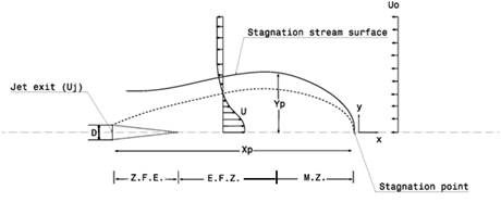
The formation of large scale vortical structures due to the strong shear layers between the jet and opposed flow creates random oscillations with large amplitudes which cause higher spreading rates compared to other jet and flow configurations like co-flow and cross-flow jets. Although there are many publications related to the discharge of a simple round jet in a uniform counter flow, the problem of a wall jet in counter flow has not been investigated completely. This flow configuration can have potential application in mixing of fluids and cooling of the heated walls in combustion chambers. The objective of this research is measuring and studying of the flow field of a round wall jet in counter flow. For this purpose a test setup is designed and a series of experiments were conducted to find the velocity field of the wall jet in counter flow with PIV and by using four cameras to cover a large area of this complex flow. The test setup is validated with available data in the literatures for the wall jet flow in quiescent environment. The experimental procedure, data analysis and several results are discussed.

2. Experimental Setup

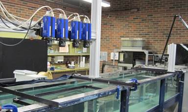
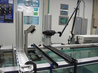
The experiments were done in the water channel facility at Mechanical Engineering Department at the University of Alberta. The size of the water channel cross section was 680×480 mm² and its total length was about 5000 mm, see Figure 3. It had a closed loop circuit and two pumps returned the water from the end plenum chamber to the front one. The volume flow rate in the water channel was adjusted by means of two valves located after each pump. It was also possible to change the height of water in the channel by adjusting the angle of a gate located at the end of the channel.  These two mechanisms were used to adjust the velocity of the flow. The water flowed from the upstream plenum chamber through an S shape nozzle with a contraction ratio of 2 and after passing from a flow straightener entered the channel. The flow straightener width was 90 mm which was made from thin copper sheet and had a mesh size of about 20×20 mm². A grid turbulence generator was located about 150 mm in front of the flow straightener.  The grid turbulence generator was made from stainless steel bars with width of 20 mm and thickness of 4 mm and had a mesh size of about 55×55 mm². 

A periscope located after the turbulence generator was used to reflect the laser sheet in the channel from the upstream. In this experiment the channel flow velocity was set to be equal to U₀ = 4cm/s and the turbulence intensity was about 3.5 %.

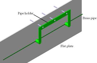
A flat plate made from acrylic with size of 400×2000 mm² was installed in the side wall of the channel far from the channel boundary layer. The distance of the flat plate leading edge was about 2m from the beginning of the channel test section and had a chamfer upstream to minimize the stagnation area. It also was equipped with a trip strip to ensure a turbulent boundary layer with a set leading edge.  The plate was equipped with a brass pipe with inner diameter equal to D = 8.84 mm and thickness of 0.1 mm to provide the jet flow in opposite direction of the channel flow, as shown in figure 4. The length of the pipe was 920 mm (104 D) which provided a fully developed flow in the pipe end. The brass pipe was held parallel to the flat plate and in the middle height by a simple supporting bar. The distance of the jet exit plane from the leading edge of the flat plate was 1200 mm. The jet discharge plane was about 40 cm far from the anchoring point to the pipe holder unit. Therefore, the interference effect of the pipe holder in the jet and opposed flow was negligible.

The jet was fed by a pressurized stainless steel tank and the channel water was used to fill the tank during the experiments. The compressed air pressure in the tank was always about 350 kPa. At the beginning of the brass pipe a flow straightener was installed to suppress any secondary flow or vortices before entering the brass pipe. It consists of a set of straws with length of 120 mm and diameter of 2 mm located in a tube with diameter of 25 mm. this tube was connected to the brass pipe by a smooth converging nozzle. A flexible hose with approximate length of 5m and inner diameter of 25mm was used to connect the pressurized tank to the flow straightener. A flow controller was installed on the jet feeding line to set the jet discharge velocity during the tests. That was a LCR-5LPM series of precise flow controllers made by Alicat Scientific Company. In this study the range of variation for velocity ratio was 1.3 < U_R < 25. The range of Reynolds number variation based on the jet diameter was about 500 < Re < 10,000.

To find the velocity field, particle image velocimetry (PIV) was used. PIV is a non intrusive technique for measuring the velocity field in a flow. It appeared about 30 years ago and is an essential measurement technique in fluid dynamics researches. In this research four cameras were used and the resultant velocity field from them were combined to have a large field of view covering the whole penetrating length of the jet. The cameras were ImagerProX4M with data depth of 14 bits and resolution of 2048×2048 pixels equipped with Nikon AF NIKKOR lenses with focal length of 50 mm. They were located in a line such that their fields of view had about 15 mm overlap with each other, see Figure 3. With the set of lenses were used in this study, the field of view for each camera was about 190×190 mm². Therefore, combining the images from these cameras provided a total field of view of 720×180 mm² which was large enough to cover the whole penetration region of the jet in counter-flow. A glass screen was installed on the water channel to have contact with the water surface to suppress the waves.

Illumination were provided by a dual cavity Nd:YAG laser with wave length of 532 nm. The laser was a Quanta Ray PIV- 400 series made by Spectra Physics and had a maximum energy of about 100 mJ in each pulse at 10 Hz repeating rate. The laser beam was transferred to the sheet generator with a laser guiding arm. The laser sheet with a thickness of about 1 mm in the test section was provided by a cylindrical lens and was directed to the channel by means of a periscope, see Figure 5.

This should be noted that due to low velocity of the channel and very stiff and solid structure of the periscope and the mounting bars, no vibration observed in the laser sheet. The laser sheet was adjusted to be parallel to the channel floor and pass through the jet central plane. The channel flow was seeded by hollow glass spheres with mean diameter of 18 µm and to have a uniform seeding density the pressurized tank was fed by the channel flow. The PIV image recording and processing were done by Davis8.2 provided by LaVision Inc.

3. Data Acquisition

When the camera's orientation and position were fixed and the test rig was ready with all components, the calibration of cameras was done to find the geometrical mappings between the image space and the real coordinate system in the test setup. The calibration target which was used in this PIV study had a size of 740×250 mm² and was consisted of filled circles with diameter of 3 mm and centre to centre spacing of 15 mm. The calibration procedure for all 4 cameras was done simultaneously. A 3^rd order polynomial fitting was selected for the calibration and the rms of fitting errors was less than 0.1%. For the PIV image acquisition, double frame and double exposure setting was selected.

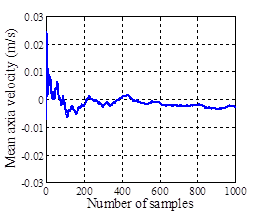
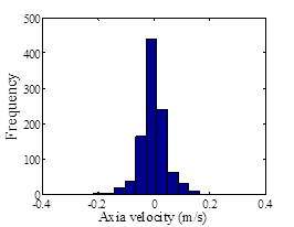
In the statistical analysis of the physical phenomena with finite data series, the number of samples is an important factor to obtain the real and accurate properties of the problem under study. In this project, finding the average behavior of the flow of a wall jet in counter-flow was the main goal. Therefore, based on the initial tests which were done before the main tests, a simple analysis was done to find how many PIV images are enough to obtain this goal. The method was to examine the behavior of the average velocity versus number of images and the distribution of velocity data at several points in the velocity field. The points were selected to be close to the shear layers of the flat plate boundary layer and the interaction zone of the jet and opposed flow in the jet boundary. Based on the physics of the problem, at these points which are shown schematically in figure 6 the velocity has more fluctuations.

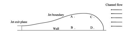
The results for point D are shown in figure 7 for the case where the jet to counter-flow velocity ratio was U_R= 20. It is seen that almost before 1000 images the average velocity approaches to a constant value or predictable behavior. Data distribution also shows that the recorded samples are acceptable since the major portion of them bouncing around the mean value. This trend was observed for points A, B, and C, too. Therefore, 1000 PIV images were recorded at each velocity ratio to obtain a valid average flow field of the wall jet in counter-flow.

In PIV experiments the setting of the time interval between the frames is an important issue which is depended on the physics of the flow and the processing scheme. Based on Davis manuals, the time difference between the images must be such that the displacement of identical particles in the image space is greater than 0.1 pixel and less than 25% of the interrogation window size. In the current experiments, the velocity field has areas with high velocity (e.g. at the jet discharge zone) and areas which the velocity vanishes (e.g. close to the wall or stagnation areas at the end of the jet penetration). Therefore, it was decided to do the experiments with one small time interval (~ 400 µs) suitable for the high velocity regions and one large time interval (3000 µs) to capture the velocity in low speed zones of the flow field. Then in the post processing of the data these two velocity field were combined with each other to find the whole velocity field.

4. Data Processing

Data processing was done by Davis 8.2 on a graphics processing unit (GPU) with total number of 1536 cores. Different schemes were selected and tested to find the most efficient and accurate scheme with lower amount of spurious vectors. Different multi-pass sequential cross correlations with decreasing window size were examined. Finally, the interrogation window size of 64×64 pixels with 50% overlap and 4 passes followed by a 16×16 pixels window size with 50% overlap and 3 passes was selected. With this processing scheme, it was found that the spatial resolution of the vector field is about 0.73×0.73 mm². This processing scheme was used to find the whole velocity field in this experimental study. In the vector post processing section, just a median filter was applied to get rid of the spurious vectors and fill the empty areas with the interpolation of neighbor vectors. Then, the average flow filed was found for each field of view. The next step was stitching the flow fields of the cameras to each other to find the total flow field of the interaction of the jet and counter-flow. Since the field of view of the cameras had overlap with each other, this overlap was found and taken out during the stitching process. A simple schematic of the cameras field of view and their overlap is shown in figure 8.

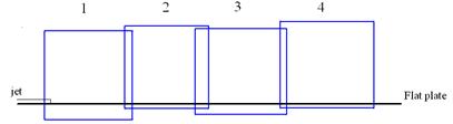
Camera 1 Camera 2 Camera 3 Camera 4

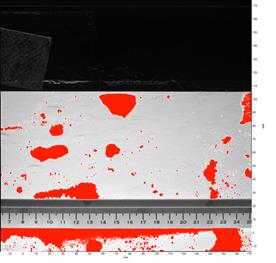
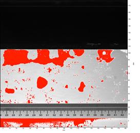
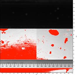
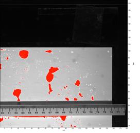
The vector fields were imported to MATLAB for stitching and further post processing. The exact amount of the overlap of cameras was found by investigating the image of a measuring tape located in the same plane where the PIV images were taken, see Figure 9. Searching was done on the images of the measuring tape from 4 cameras to find the common values. After finding the amount of overlaps, the images were cut with pixel accuracy to get rid of the common areas. This procedure was repeated for all velocity fields captured by each camera. So, for each data set the final velocity vector was extracted and used for further analysis.

The precision error in the measurement of the velocity field was estimated to be around 0.3%.  In order to reduce the bias errors, the rules of thumb mentioned by Raffel et al. [13] was followed. The total amount of uncertainty in the mean velocity measurement was evaluated to be around 2.5%.

5. Results

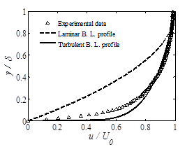
An experiment is designed to measure the velocity field of a wall jet in counter-flow at different jet to counter-flow velocity ratios, up to U_R = 25. The main boundary conditions in this flow field are related to the counter-current flow, the boundary layer of the flat plate, and the jet outlet velocity. The flow condition of the channel was a uniform flow with the velocity of 4 cm/s and turbulence intensity of 3.5%. The boundary layer of the flat plate was tripped to be turbulent by a guitar string installed at a distance of 100 mm after the plate leading edge. The normalized velocity profile in the boundary layer of the plate at a distance of x = 25 D from the jet outlet plane is shown in Figure 10 a. The typical laminar and turbulent boundary layer profiles over flat plates described by Schlichting [14] are shown for comparison.  It is clear that the experimental boundary layer velocity profile is similar to the turbulent profile; the discrepancy is due to the low Reynolds number artificially transitioned flow in these experiments.

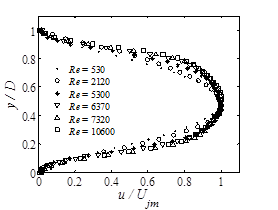
Detailed jet velocity profiles were obtained for the free jet exiting the brass pipe in the absence of the flat plate. Figure 10 b shows the normalized mean axial velocity profiles at different Reynolds numbers based on the jet diameter at a distance of 0.4 D from the outlet plane. It is seen that with increasing Reynolds number, the velocity profiles become fill out like a turbulent pipe flow and show minimal variation for Re > 5000. It will be shown later that at low Reynolds number, the jet velocity decay starts at a greater distance from the discharge plane.

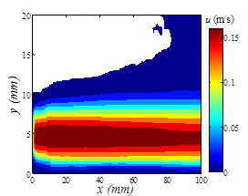
In order to ensure the capability and accuracy of this test setup, initial experiments were done to measure the velocity field of the wall jet when the water channel was not running. The results were then compared with the existing data in the literatures for three dimensional round wall jets in quiescent ambient. Figure 11 shows a small portion of the axial velocity contour of the round wall jet at Re =1,000 and Re = 9,500. It is seen that at lower Reynolds number, the axial velocity decay is very slow and there is a long core in which the velocity is almost constant. At the initial region, the jet shows laminar behavior and after a certain distance it becomes turbulent. On the other hand, when the Reynolds number is high enough, the jet velocity decay starts immediately after the jet exit and the jet is completely turbulent, see Figure 11b.

The normalized maximum velocity decay of the wall jet versus axial distance is shown in figure 12a for range of Reynolds numbers from Re = 2,000 to 10,000. It is seen that for Re >7.3×10³ the velocity profiles collapse on each other and show self similar behavior. Figure 11b shows that for the self similar velocity decay and axial distances of x/D >15, a power law relation (R²=95%) can be used to represent the velocity distribution in the form of:

Um / Ujm = 8.5 (x / D)-1.08

(2)

where U_m is the maximum wall jet axial velocity, and U_jm is the maximum jet discharge velocity. This result has agreement with previous research of Law and Herlina [3] in which they found -1.07 power law fit for the velocity decay of a three dimensional wall jet provided by a round nozzle.

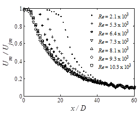
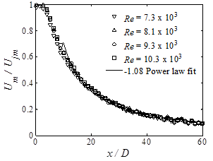
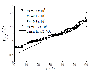
Figure 13 shows the variation of half velocity width (y_1/2) of the round wall jet versus axial distance from the jet exit plane. For x /  D > 30, it is seen that the variation of jet width is linear with slope of 0.04. Therefore, a linear fit (R²=95%) for the half width velocity of the round wall jet can be proposed as:

y1/2 / D = 0.5 + 0.04 (x / D)

(3)

The normalized axial velocity distribution of the wall jet at two different Reynolds numbers and several distances downstream of the discharge plane is shown in figure 14. The velocity profiles show self similarity for x / D > 30. As figure 14 shows, the velocity profile proposed by Verhoff [15] can completely represent the current experimental data. This velocity profile is in the form of:

u / Um = 1.48 (y / y1/2)1/7 [1-erf (0.68 ( y / y1/2 ))]

(4)

where u is the axial velocity at the local region.

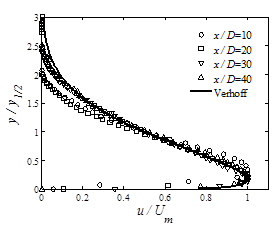
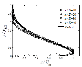
From the above results one can conclude that the measured velocity field of the round wall jet in still ambient has complete agreement with similar experiments done by other researchers. This proves the capabilities of the designed test setup for measuring the velocity field of the round wall jet with the presence of the counter-flowing stream in the water channel.

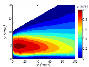
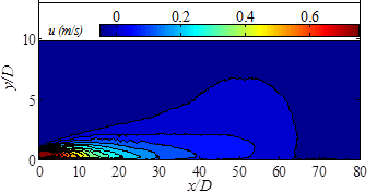
The whole flow field for the wall jet in counter-flow at U_R = 17.5 corresponding to jet Reynolds number of Re  =7,300 is shown in figures 15.  As it is seen, the jet penetrates and exchange momentum with the counter-flow and finally reaches to zero velocity at maximum penetration length of  X_p = 64 D.

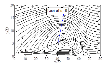
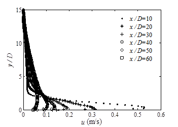
Figure 16 shows a schematic of the stream lines in a 2-D plane along with the loci of u = 0 regions. It clearly shows the path of fluid elements toward the stagnation area and their turning. There is a recirculation region close to the stagnation area which contains a big swirl at x/D = 48. The axial velocity profiles at different positions are shown in figure 17. It is seen that the profiles have a typical shape of a wall jet flow at initial regions. Then, the quick decay of axial velocity profile starts around x/D = 40 and continues to reach to zero velocity at maximum penetration point. Different length scales of the flow can be used to normalize these velocity profiles like what was done for a wall jet in quiescent environment.

6. Conclusion

The purpose of this research was to design an experimental procedure for studying the behavior of a round wall jet in counter-flow. The wall jet and counter-flowing jet were defined and their typical applications were discussed briefly. The velocity field of a three dimensional round wall jet exiting from a pipe is analyzed at different Reynolds numbers ranging from 500 to 10,000 for still ambient. The results show complete agreement with available information in the literatures. The self-similarity of wall jet velocity data was observed for Re >7,000. The maximum velocity decays with power of -1.08 versus the axial distance and the normalized axial velocity profiles collapse on each other for x/D > 30. The velocity field of the wall jet in counter-flow at velocity ratio of U_R= 17.5 is discussed shortly. It was observed that the jet penetrates up to x/D =64 and there exist a large recirculation region close to the stagnation area.

References

[1] B.E. Lander, and W. Rodi, "The turbulent wall jet- Measurement and modeling," Annual Review of Fluid Mechanics, 15, 1983, pp. 429-459. View Article
[2] J.G. Eriksson, R.I. Karlsson, andJ. Persson, "An experimental study of a two-dimensional plane turbulent wall jet," Experiments in Fluids, 25, 1998, pp. 50-60. View Article
[3] A.W. Law, and Herlina, "An experimental study on turbulent circular wall jets," Journal of Hydraulic Engineering, 128, 2002, pp. 161-174. View Article
[4] M. Yoda, H.E. Fiedler, "The Round Jet in a Uniform Counter-Flow: Flow Visu¬alization and Mean Concentration Measurements", Experiments in Fluids, 21(6), 1996, pp. 427- 436. View Article
[5] H.C. Chan, K.M. Lam, "Centerline Velocity Decay of a Circular Jet in a Counter-Flowing Stream", Physics of Fluids, 10(3), 1998, pp. 637-644. View Article
[6] L.A. Torres, M. Mahmoudi, B.A. Fleck, D.J. Wilson, D.S. Nobes, "Mean Concentration Field of a Jet in a Uniform Counter-flow", Journal of Fluid Engineering 134, 2012, 14502-1 - 5. View Article
[7] O. Konig and H.E. Fiedler, "The Structure of Round Turbulent Jets in Counter-Flow: a Flow Visualization Study," Advances in Turbulence 3, 1991, pp. 61-66. View Article
[8] J.S. Shang, "Validation of plasma injection for hypersonic blunt-body drag reduction," RTO AVT Symposium On Reduction Of Military Vehicle Acquisition Time And Cost Through Advanced Modelling And Virtual Simulation, Paris, France, 2002, April 22-25. View Article
[9] R. Sriram, and G. Jagadeesh, "Film cooling at hypersonic Mach numbers using forward facing array of micro-jets," International Journal of Heat and Mass Transfer, 52, 2009, pp.3654–3664. View Article
[10] G. Balla Venukumar, K.P. Jagadeesh, and J. Reddy, "Counter-flow drag reduction by a supersonic jet for a blunt body in hypersonic flow," Physics of Fluids, 18, 2006. View Article
[11] A. Khamooshi, T. Taylor, and D. Riggins, "Innovative Concepts for Large-Scale Drag and Heat Transfer Reduction in High-Speed Flows," AIAA Journal, 45(10), 2007, pp. 2401-2413. View Article
[12] C.M. Or, K.M. Lam, P. Liu, "Potential core lengths of round jets in stagnant and moving environments" Journal of Hydro-environment Research 5, 2011 pp. 81-91. View Article
[13] M. Raffel, C.E. Willert and J. Kompenhaus, "Particle Image Velocimetry: A Practical Guide," Springer Verlag, 1998. View Book
[14] H. Schilichting, "Boundary Layer Theory," McGraw-Hill, 4th edition, 1962. View Article
[15] A. Verhoff, "The two-dimensional turbulent wall jet with and without an external stream," Rep. No. 626, Princeton University, Princeton, N.J., 1963.