International Journal of Mechanical Engineering and Mechatronics (IJMEM)
ISSN: 1929-2724

Volume 1, Issue 2 Year 2012 - Pages 50-60
DOI: 10.11159/ijmem.2012.006
LMI-based Adaptive Observers for Nonlinear Systems
Jiang Zhu, Karim Khayati
Royal Military College of Canada, Department of Mechanical & Aerospace Engineering Po Box 17000, Station Forces,
Kingston, Ontario, Canada K7K 7B4
jiang.zhu@rmc.ca; karim.khayati@rmc.ca
Abstract - This paper deals with the design of adaptive observers that can estimate both the states and the parameters of a large class of nominal and perturbed nonlinear systems with a regression matrix (i.e. matching matrix with the unknown parameter vector) depending on unknown states. The asymptotic stability of the state and parameter estimate errors is developed in the presence of common persistency of excitation (PE). The observer gain calculus is cast as a linear matrix inequality (LMI) feasibility problem. The appeal of this proven theoretical design is further demonstrated numerically.
Keywords: Nonlinear System, Perturbed Dynamics, Adaptive Observer, Parameter Estimation, LMI.
© Copyright 2012 Authors - This is an Open Access article published under the Creative Commons Attribution License terms. Unrestricted use, distribution, and reproduction in any medium are permitted, provided the original work is properly cited.
1. Introduction
The adaptive observer design for linear and nonlinear systems has been widely investigated during the last few decades (Khayati & Zhu, 2011; Zhu & Khayati, 2011; Maatoug et al., 2008; Cho & Rajamani, 1997; Marino & Tomei, 1995) and references cited therein. In (Cho and Rajamani, 1997), the authors have designed a systematic approach for an adaptive observer that estimates the full-state variables for nonlinear dynamics in the presence of uncertain parameters possibly depending on the input and state variables. The stability of the algorithm is guaranteed when at least some of the measured outputs are such that the transfer matrix from the unknown parameters to these outputs is dissipative (Cho & Rajamani, 1997). The design of the observer depends on the ability to solve an LMI problem under a conservative matrix equality refering to "matchning conditions" of the dynamic representation. Even, it has been reported and applied in many other works in the literature (Dimassi et al., 2010; Liu, 2009; Dong & Mei, 2007; Stepanyan & Hovakimyan, 2007; Zhu, 2007), this concept is still hard to achieve within some (but very common) dynamics as discussed in (Zhu and Khayati, 2011).
The design of adaptive observer schemes to estimate jointly the states and the parameters for nonlinear dynamic systems with uncertainties referring more to actual scenarios has been studied (Dimassi et al., 2010; Liu, 2009; Marino et al., 2001). However, there are still problems (other than the matching conditions) in these given adaptive observers, and also, the assumptions are difficult to achieve (Dimassi et al., 2010) (Dimassi et al., 2010; Liu, 2009). In most of these recent works, authors have considered the case of known nonlinear regression matrix of measurable states and inputs (Zhao et al., 2011; Paesa et al., 2010; Zemouche & Boutayeba, 2009; Garimella & Yao, 2003; Marino et al., 2001). In (Zemouche & Boutayeba, 2009), a unified H∞ adaptive observer for a class of nonlinear systems is introduced to estimate uncertain parameters in the unmeasured nonlinearities. These nonlinearities are limited to monotonic functions. In (Stamnes et al., 2009), the authors have designed a nonlinear adaptive observer for a limited class of nonlinear systems. The proposed adaptation law has been built using nonlinear partial differential equations in known and unknown states. However, the stability of such an observer requires nonlinear time-varying "sector conditions" to be satisfied.
In this paper, a more general form of the adaptive observer scheme discussed in (Zhu and Khayati, 2011) will be extended to nonlinear dynamics with a regression matrix function of both measurable and unmeasurable signals and unknown disturbances. The stability condition of the proposed adaptive observer will be presented using only strict LMIs (Boyd et al., 1994). The proposed design estimating the full states and identifying the unknown parameters for a large class of nonlinear dynamic systems is cast with general conditions that are still feasible and address realistic plants. This paper is organized as follows. In Section 2, we describe the problem statement and assumptions. In Section 3, we introduce the general form of the nonlinear adaptive observer (NLAO) for the nominal dynamics (with no disturbances), and then, the robust nonlinear adaptive observer (RNAO) for perturbed nonlinear dynamics respectively. Section 4 shows illustrative simulation examples, while Section 5 concludes this work.
2. Statement and Assumptions
Problem Statement
Consider the nonlinear dynamics with unknown disturbances:
|
|
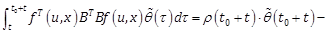
(1) |

|
|
(2) |

where![]() is the state vector,
is the state vector, ![]() the input vector,
the input vector, ![]() the output,
the output, ![]() the vector of unknown constant parameters and
the vector of unknown constant parameters and ![]() represents unknown disturbances.
represents unknown disturbances. ![]() ,
, ![]() ,
, ![]() ,
, ![]() ,
, ![]() ,
, ![]() and
and ![]() are known constant
matrices.
are known constant
matrices. ![]() ,
, ![]() and
and ![]() are nonlinear functions in
are nonlinear functions in![]() ,
, ![]() and
and![]() , respectively.
, respectively.
Assumptions
For the forthcoming design, we consider the following assumptions (Zhu and Khayati, 2011):
A1.The
vector of unknown constant parameters ![]() is
bounded, with
is
bounded, with
|
|
(3) |

A2.![]() is
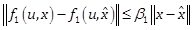
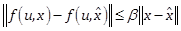
continuously bounded, and both functions
is
continuously bounded, and both functions ![]() and
and ![]() are
Lipschitz in
are
Lipschitz in![]() , with
, with
|
|
(4) |
|
|
(5) |
A3.The input
vector ![]() is of class
is of class ![]() (i.e. continuous function having continuous first derivatives).
(i.e. continuous function having continuous first derivatives).
3. Adaptive Observer Design
For the adaptive observer design, we first briefly introduce the design for the case of nominal dynamics i.e. disturbance free one; then we extend it to the perturbed case and prove the effectiveness.
3.1. Case 1 – Nominal Dynamics
Given the unperturbed nonlinear model, that is described by (1) and
(2) with ![]() and
and
![]() . Consider the following full-order nonlinear observer
. Consider the following full-order nonlinear observer
|
|
(6) |

and adaptation law
|
|
(7) |

|
|
(8) |
where ![]() is the total time
derivative of
is the total time
derivative of ![]() given by
given by ![]() ,
, ![]() matrix
of
matrix
of ![]() ,
, ![]() ,
, ![]() and
and ![]() matrices
of
matrices
of ![]() .
.
Proposition 1 – Under assumptions A1-A3, if there exist matrices ![]() in
in ![]() and
and
![]() such that
such that
|
|
(9) |
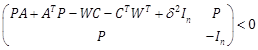
with ![]() and matrices
and matrices ![]() and
and ![]() of
of
![]() computed from
computed from
|
|
(10) |

with ![]() the identity
matrix of
the identity
matrix of ![]() , then the state estimation error
vector
, then the state estimation error
vector ![]() of the NLAO (6)-(8), with the observer gain matrix computed
as
of the NLAO (6)-(8), with the observer gain matrix computed
as ![]() , for the nominal system (1) and (2) tends to zero and the parameter estimate error vector
, for the nominal system (1) and (2) tends to zero and the parameter estimate error vector ![]() is radially bounded. In
addition, if for some positive scalars
is radially bounded. In
addition, if for some positive scalars ![]() ,
, ![]() and
and ![]() with
the inequalities
with
the inequalities
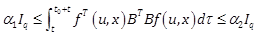
|
|
(11) |
hold ![]() , where
, where ![]() is the identity matrix of order
is the identity matrix of order ![]() , then both estimate errors
, then both estimate errors ![]() and
and ![]() asymptotically
as
asymptotically
as ![]() . The condition (11) refers to the PE which is very common in the literature (Maatoug et al., 2008; Dong & Mei, 2007; Cho
& Rajamani, 1997).
. The condition (11) refers to the PE which is very common in the literature (Maatoug et al., 2008; Dong & Mei, 2007; Cho
& Rajamani, 1997).
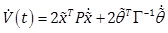
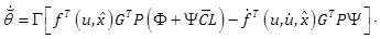
Proof – Let ![]() and
and ![]() be
the state and parameter estimate errors, respectively. From (1), (2) and (6), we derive
be
the state and parameter estimate errors, respectively. From (1), (2) and (6), we derive
|
|
(12) |


|
|
(13) |


By using the conditions (10), (13) reduces to
|
|
(14) |
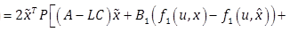
Now, to investigate the stability, given ![]() and
and ![]() ,
consider the Lyapunov candidate function
,
consider the Lyapunov candidate function ![]() (Khayati
and Zhu, 2011). Using (12) and (14), we have
(Khayati
and Zhu, 2011). Using (12) and (14), we have
|
|
(15) |
|
|
(16) |
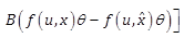
Using ![]() , we notice the
inequality
, we notice the
inequality ![]() , we obtain
, we obtain
|
|
(17) |
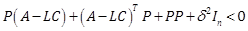
![]() is negative if
is negative if
|
|
(18) |
The inequality (18), which is nonlinear in ![]() and
and
![]() (nonlinearities refer to
(nonlinearities refer to ![]() and
and ![]() ),
will be transformed into the LMI (9) by simply applying the Schur complement
theorem (Boyd et al. 1994) and the change of variable
),
will be transformed into the LMI (9) by simply applying the Schur complement
theorem (Boyd et al. 1994) and the change of variable ![]() .
.
Now, from (17) and (18), ![]() such that
such that
|
|
(19) |

This implies ![]() (i.e.
time-functions of finite ¥-norm), and
then
(i.e.
time-functions of finite ¥-norm), and
then ![]() and
and ![]() . Integrating
(19) leads to
. Integrating
(19) leads to
|
|
(20) |
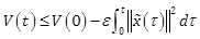
Since ![]() is finite, we obtain
is finite, we obtain ![]() (i.e.
finite 2-norm vector-function).
From (12), we have
(i.e.
finite 2-norm vector-function).
From (12), we have ![]() . Therefore, by applying theorem 8.4 of (Khalil, 2002) based on Barbalat's Lemma,
. Therefore, by applying theorem 8.4 of (Khalil, 2002) based on Barbalat's Lemma, ![]() and
and ![]() . From (12), we have
. From (12), we have ![]() . Using the inequality (5) and noting that
. Using the inequality (5) and noting that ![]() , we have
, we have ![]() . So, from
. So, from ![]() and
and ![]() is constant (i.e. assumption
A1), we obtain
is constant (i.e. assumption
A1), we obtain ![]() and then
and then ![]() as
as ![]() (Dong and Mei 2007). Hence,
(Dong and Mei 2007). Hence, ![]() as
as ![]() . In the following, we investigate the PE
property to lead to
. In the following, we investigate the PE
property to lead to ![]() . Define
. Define ![]() (Dong and Mei 2007). Using the integration by parts,
we obtain
(Dong and Mei 2007). Using the integration by parts,
we obtain
|
|
(21) |
As ![]() , we obtain
, we obtain
|
|
(22) |
Since ![]() , then for any
finite
, then for any
finite ![]() , we have
, we have
|
|
(23) |

Moreover, since ![]() is
bounded (see assumption A2) and
is
bounded (see assumption A2) and ![]() , from (14), we have
, from (14), we have ![]() , and then
, and then ![]() as
as ![]() .
Thus, from (22), we have
.
Thus, from (22), we have ![]() ,
as
,
as ![]() . From the assumption of PE (11), i.e.
. From the assumption of PE (11), i.e. ![]()
![]() for positive scalars
for positive scalars ![]() and
and
![]() , we obtain
, we obtain ![]() ,
implying
,
implying ![]() (Dong
& Mei, 2007).
(Dong
& Mei, 2007).
3.2. Case 2 – Perturbed Dynamics
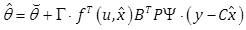
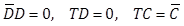
Consider the perturbed dynamics (1) and (2) under assumptions A1-A3. We propose the following RNAO scheme
|
|
(24) |


|
|
(25) |
|
|
(26) |

|
|
(27) |

where ![]() is the total time
derivative of
is the total time
derivative of ![]() ;
; ![]() ,
,
![]() ,
, ![]() ,
, ![]() ,
, ![]() ,
, ![]() ,
, ![]() ,
, ![]() ,
, ![]() and
and
![]() are constant matrices computed by the
following
are constant matrices computed by the
following
|
|
(28) |

|
|
(29) |
|
|
(30) |

|
|
(31) |

with ![]() being the identity
matrix of
being the identity
matrix of ![]() ,
, ![]() the
observer gain and
the
observer gain and ![]() the adaptation matrix gain
of
the adaptation matrix gain
of ![]() .
.
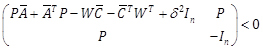
Proposition 2 – Under assumptions A1-A3, if there exist matrices ![]() in
in ![]() and
and
![]() such that (32) holds, then
such that (32) holds, then ![]() and
and
![]() is radially bounded as
is radially bounded as ![]() .
.
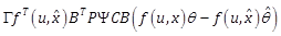
|
|
(32) |

with ![]() . The observer
gain matrix is
. The observer
gain matrix is ![]() . The algebraic equality
conditions (28)-(31) complete the computation of the adaptive observer
scheme. In addition, if the PE condition
. The algebraic equality
conditions (28)-(31) complete the computation of the adaptive observer
scheme. In addition, if the PE condition
|
|
(33) |
holds for some positive scalars ![]() ,
, ![]() and
and
![]() , then the RNAO (24)-((27)) for the
perturbed dynamics (1) and (2) is asymptotically stable, that is both
state and parameter estimates converge asymptotically to their actual values as
, then the RNAO (24)-((27)) for the
perturbed dynamics (1) and (2) is asymptotically stable, that is both
state and parameter estimates converge asymptotically to their actual values as
![]() .
.
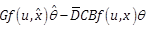
Proof – Using ![]() , the observer output is
reduced to
, the observer output is
reduced to ![]() . Its time derivative is then obtained
from (1), (2), (24), (25) and
. Its time derivative is then obtained
from (1), (2), (24), (25) and ![]()
|
|
(34) |


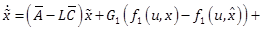
Let ![]() be the state
estimate error. From (1), (2), (24), (25), we derive
be the state
estimate error. From (1), (2), (24), (25), we derive
|
|
(35) |

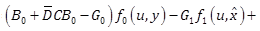
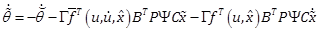
Using (29) and (30), we obtain
|
|
(36) |

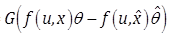
From (26) and (27), using ![]() and the error
dynamics (36), we derive
and the error
dynamics (36), we derive
|
|
(37) |


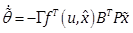
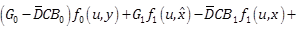
By using the conditions (31), the dynamics (37) reduces to
|
|
(38) |
Let ![]() be the parameter estimate
error. Based on assumption A1, we have the
be the parameter estimate
error. Based on assumption A1, we have the ![]() .
Then, we obtain the adaptation error dynamics
.
Then, we obtain the adaptation error dynamics
|
|
(39) |

To investigate the stability of the estimate error
dynamics and the proposed LMI feasibility problem, we consider the same
Lyapunov function ![]() and the PE condition (33), and we follow the same steps of the proof of Proposition 1 shown
above.
and the PE condition (33), and we follow the same steps of the proof of Proposition 1 shown
above.
3.3 Comments
In the first algorithm, we discuss a nonlinear
adaptive observer for disturbance-free dynamics with nonlinear regression
matrix function of unknown states. The
proposed design has the advantage of being applied appropriately for nonlinear
dynamics (1)-(2)
with the particular property of ![]() ; that is, columns
of the matrix
; that is, columns
of the matrix ![]() lie in the null space of
the output matrix
lie in the null space of
the output matrix ![]() .
.
Then, we consider the more general case of perturbed nonlinear dynamics. The proposed observer in the second scheme decouples the effect of the disturbances from the estimation process. This scheme is expected to improve the accuracy and robustness of estimation when the system is subject to unknown disturbances and noisy measurement. Both schemes represent a generalization of the second order adaptive observer dynamics introduced in (Zhu & Khayati, 2011). The key element of the proposed design is inspired by (Zhao et al., 2011) where the authors have considered only a linear dynamics counterpart with a known regression term.
The matrices of the adaptive observers are computed using equations and LMIs, independently. These independent computations make the design of the NLAO and RNAO feasible provided the common assumptions and the LMI (9) (or (32)) are satisfied. This design is more tractable numerically than the method in (Cho & Rajamani, 1997) which needs more effort to solve a set of equalities and inequalities simultanously.
4. Illustrative examples
In this section, we show three illustrations enhancing the effectiveness of both schemes discussed above. The first example shows a low speed motion with a dynamic friction of unknown states and parameters. In the second example, we consider a disturbed second order mechanical dynamics with nonlinear terms, while the third one represents a third order dynamics including an uncertain nonlinear term.
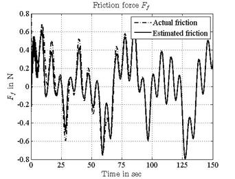
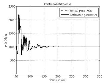
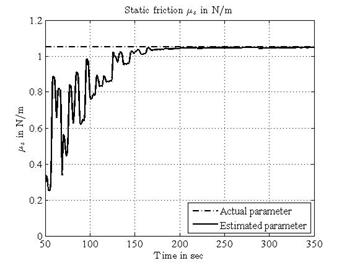
4.1 Example 1 – Low speed motion with dynamic friction
Consider a single known mass ![]() at position
at position ![]()
|
|
(40) |

under the influence of a dynamic friction ![]() and an input force
and an input force ![]() . The friction force
. The friction force ![]() is given by the modified LuGre model:
is given by the modified LuGre model:
|
|
(41) |

|
|
(42) |
where ![]() with
with ![]() represents the actual velocity.
represents the actual velocity. ![]() is the frictional stiffness.
is the frictional stiffness. ![]() is the normalized Coulomb friction
and
is the normalized Coulomb friction
and ![]() the normalized static friction
coefficient. The parameters
the normalized static friction
coefficient. The parameters ![]() ,
, ![]() and
and ![]() are
unknown. We assume the position
are
unknown. We assume the position ![]() and the velocity
and the velocity ![]() are both measurable, but
are both measurable, but ![]() is unknown and is under the
stiffness, Stribeck, static and Coulomb effects in the absence of internal and
external damping frictions (Canudas et
al., 1995). The term
is unknown and is under the
stiffness, Stribeck, static and Coulomb effects in the absence of internal and
external damping frictions (Canudas et
al., 1995). The term ![]() represents a finite function which is
chosen to describe the different friction effects. It replaces the function
given in (Canudas et al., 1995):
represents a finite function which is
chosen to describe the different friction effects. It replaces the function
given in (Canudas et al., 1995):
|
|
(43) |

In the literature, it was widely proven that the
friction parameterization is not limited to (43). Indeed, this term is nonlinear in the unknown parameter. By using (42), the proposed modified LuGre model presents an
easy-to-use linear-in-the-parameters form that captures most of the observed
static friction phenomena of velocity and the unknown parameters become linearly
dependent and thus suitable for any on-line estimation. ![]() denotes
the Stribeck time constant and indicates the velocity range in which the
Stribeck effect is effective. The friction model is a nonlinear function of
denotes
the Stribeck time constant and indicates the velocity range in which the
Stribeck effect is effective. The friction model is a nonlinear function of ![]() . To prevent further difficulties with
the nonlinear estimation technique, an empirical value of
. To prevent further difficulties with
the nonlinear estimation technique, an empirical value of ![]() is selected from the literatures (Waiboer et al., 2005; Canudas et al.,
1995). The state
representation
is selected from the literatures (Waiboer et al., 2005; Canudas et al.,
1995). The state
representation ![]() ,
, ![]() ,
,
![]() and
and ![]() defines
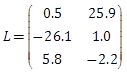
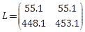
the system in the state space form (1) and (2) using the model matrices shown in Table 1. For
simulation purposes, the parameters characterizing the mechanical system are
chosen
defines
the system in the state space form (1) and (2) using the model matrices shown in Table 1. For
simulation purposes, the parameters characterizing the mechanical system are
chosen ![]() ,
, ![]() ,
, ![]() ,
, ![]() and
and
![]() respectively. The unknown parameters
are
respectively. The unknown parameters
are ![]() ,
, ![]() ,
and
,
and ![]() , respectively. To estimate the
unknown friction force and parameters, we apply the NLAO design with the
computed parameters as shown in Table 1. The estimates of the states are shown in
Figures 1-3. The
estimates of the parameters are depicted in Figures 4-6. Both
the state estimation error and the parameter error converge to zero quickly and
accurately.
, respectively. To estimate the
unknown friction force and parameters, we apply the NLAO design with the
computed parameters as shown in Table 1. The estimates of the states are shown in
Figures 1-3. The
estimates of the parameters are depicted in Figures 4-6. Both
the state estimation error and the parameter error converge to zero quickly and
accurately.
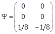
Table 1. Plant and NLAO parameters in example 1.
|
Plant |
|
|
NALO |
|
 ,
,  ,
,  ,
,
 ,
, 
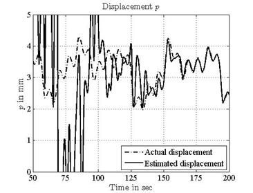
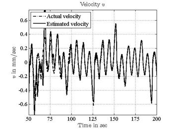
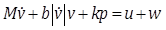
4.2. Example 2 – Nonlinear mass-spring-damper (MSD) model
We consider the MSD model introduced in (Stamnes et al., 2009)
|
|
(44) |
where ![]() is the applied
force,
is the applied
force, ![]() the position and
the position and ![]() the velocity,
the velocity, ![]() a
load disturbance. The positive constants
a
load disturbance. The positive constants ![]() ,
, ![]() and
and ![]() are
unknown and denote the spring stiffness, the mass, and the nonlinear damping
coefficient, respectively. We assume the position and the velocity measurements
are both available but with some noise affecting the velocity signal. By
assuming the fact that the load exhibit some noisy disturbance with similar
frequency spectra, for simplicity we consider that both load and measurement
noises have the same magnitude. Using the states
are
unknown and denote the spring stiffness, the mass, and the nonlinear damping
coefficient, respectively. We assume the position and the velocity measurements
are both available but with some noise affecting the velocity signal. By
assuming the fact that the load exhibit some noisy disturbance with similar
frequency spectra, for simplicity we consider that both load and measurement
noises have the same magnitude. Using the states ![]() and
and
![]() and the output vector components
and the output vector components ![]() and
and ![]() ,
this dynamic model can be written in the state space representation (1) and (2) using the model matrices shown in Table 2.
The components of the unknown vector
,
this dynamic model can be written in the state space representation (1) and (2) using the model matrices shown in Table 2.
The components of the unknown vector ![]() are
are ![]() ,
, ![]() and
and
![]() , respectively (Stamnes et al., 2009). The parameters characterizing the simulated MSD
dynamics are chosen
, respectively (Stamnes et al., 2009). The parameters characterizing the simulated MSD
dynamics are chosen ![]() ,
, ![]() and
and
![]() , respectively. To estimate the
unknown states and parameters of the dynamics, we consider first the nominal
case by assuming a disturbance free dynamics and we apply the NLAO scheme.
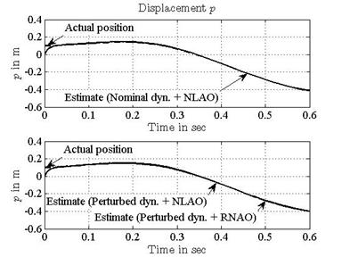
Then, we consider the perturbed dynamics for which we apply both the NLAO and
RNAO and compare their effectiveness and performances. The observer and
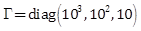
adaptation law parameters of the NLAO (6)-(8) and the RNAO (24)-(27) are obtained in Table 2. Consider
the input signal
, respectively. To estimate the
unknown states and parameters of the dynamics, we consider first the nominal
case by assuming a disturbance free dynamics and we apply the NLAO scheme.
Then, we consider the perturbed dynamics for which we apply both the NLAO and
RNAO and compare their effectiveness and performances. The observer and
adaptation law parameters of the NLAO (6)-(8) and the RNAO (24)-(27) are obtained in Table 2. Consider
the input signal ![]() which results in
sufficiently rich input signal that guarantees the fulfillment of the PE
condition and that is necessary to ensure the convergence of the unknown
parameters to their true values). The simulation results are shown in Figures 7-11. Both the state estimation error and the
parameter error converge to zero quickly and accurately.
which results in
sufficiently rich input signal that guarantees the fulfillment of the PE
condition and that is necessary to ensure the convergence of the unknown
parameters to their true values). The simulation results are shown in Figures 7-11. Both the state estimation error and the
parameter error converge to zero quickly and accurately.
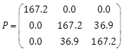
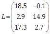
Table 2. Plant, NLAO and RNAO parameters in example 2.
|
Plant |
|
|
NALO |
|
|
RNAO |
|
 of the MSD dynamics.
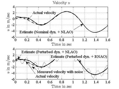
 of the MSD dynamics.
 of the MSD dynamics.
4.3. Example 3 – Nonlinear third order dynamics
Consider the dynamics below
|
|
(45) |

|
|
(46) |
|
|
(47) |

|
|
(48) |
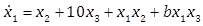
![]() and
and ![]() are the measurable states. The vector of the unknown
parameters is
are the measurable states. The vector of the unknown
parameters is ![]() . For simulation, we choose
. For simulation, we choose ![]() ,
, ![]() and
and
![]() . First, considering the nominal
dynamics, the parameter
. First, considering the nominal
dynamics, the parameter ![]() is assumed to be a
well-posed constant
is assumed to be a
well-posed constant ![]() . Thereafter, we simulate
with some dynamic perturbation by assuming
. Thereafter, we simulate
with some dynamic perturbation by assuming ![]() uncertain.
For simulation, we consider
uncertain.
For simulation, we consider ![]() . The observer and
adaptation law matrices of the NLAO and RNAO are shown in Table
3.
. The observer and
adaptation law matrices of the NLAO and RNAO are shown in Table
3.
Table 3. Plant, NLAO and RNAO parameters in example 3.
|
NALO |
|
|
RNAO |
|
 ,
,  ,
,
 ,
, 
 ,
,  ,
,  ,
,  ,
,  ,
, 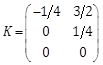 ,
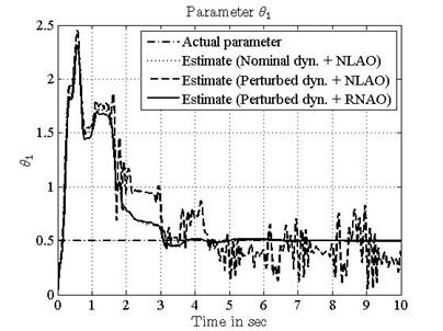
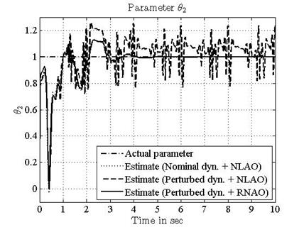
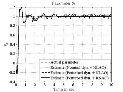
, Using a linear combination of sine waves as an input signal, all results of the estimates of the states and parameters obtained with the two proposed methods (NLAO and RNAO) are shown in Figures 12-17. Both the state estimation error and the parameter error converge to zero quickly and accurately.

 of the 3rd order
dynamics (example 3).
of the 3rd order
dynamics (example 3).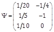
 of the 3rd order
dynamics (example 3).
of the 3rd order
dynamics (example 3).
 of the 3rd order
dynamics (example 3).
of the 3rd order
dynamics (example 3). of the 3rd order
dynamics (example 3).
of the 3rd order
dynamics (example 3). of the 3rd order
dynamics (example 3).
of the 3rd order
dynamics (example 3). of the 3rd order
dynamics (example 3).
of the 3rd order
dynamics (example 3).5. Conclusion
A new nonlinear adaptive observer and a corresponding robust scheme are derived for a wide class of nonlinear dynamic systems with unknown parameters, uncertain dynamics and disturbances. The asymptotic stability is developed using LMI frameworks. The proposed estimation design exhibits a satisfactory convergence of both the states and the parameters to the actual values. Examples with simulation results successfully demonstrate the effectiveness of the proposed schemes. It is shown that both RNAO and NLAO track the trajectory but with a difference. In fact, the NLAO design has better performance with the nominal case than the perturbed one. We depict the difference that the state estimations under the RNAO approach the actual state coincidently while the NLAO does not. Moreover, the parameter estimation errors under the RNAO converge to zero despite the presence of uncertain dynamics, but the errors under the NLAO converge to zero only when the system is nominal.
References
Boyd, S., El Ghaoui, L., Feron, E., Balakrishnan, V., (1994) Linear Matrix Inequalities in Systems and Control Theory. SIAM Studies in Applied Mathematics. View Article
Canudas, C., Olson, H., Astrom, K., Lischinsky, P., (1995). A New Model for Control of Systems with Friction. IEEE Transactionon Automatic Control, Volume 40(3), pp. 419-425. View Article
Cho, Y., Rajamani, R., (1997). A Systematic Approach to Adaptive Observer Synthesis for Nonlinear Systems. IEEE Transaction on automatic Control, Volume 42(4), pp. 534-537. View Article
Dimassi, H., Loria, A., Belghith, S., (2010). A Robust Adaptive Observer for Nonlinear Systems with Unknown Inputs and Disturbances. 49th IEEE Conference on Decision and Control, pp. 2602-2607, Atlanta, GA. View Article
Dong, Y.-L., Mei, S.-W., (2007). Adaptive Observer for a Class of Nonlinear Systems. Acta Automatica Sinica, Volume 33(10), pp. 1081-1084. View Article
Garimella, P., Yao, B., (2003). Nonlinear Adaptive robust observer design for a class of nonlinear systems. Denver, Colorado, USA, pp. 4391-4396. View Article
Khalil, H., (2002). Nonlinear Systems. 3rd Edition, Prentice-Hall, New York. View Article
Khayati, K., Zhu, J., (2011). Nonlinear Adaptive Observer Design for an Electromechanical Rotative Plant. 24th Canadian Conference Electrical and Computer Engineering, Niagara Falls, pp. 385-388. View Article
Liu, Y., (2009). Robust Adaptive Observer for Nonlinear Systems with Unmodeled Dynamics. Automatica, Volume 45, pp. 1891-1895. View Article
Maatoug, T., Farza, M., M'Saad, M., Koubaa, Y., Kamoun, M., (2008). Adaptive Observer Design for a Class of Nonlinear Systems with Coupled Structures. International Journal of Sciences and Techniques of Automatic Control,Computer Engineering, Volume 2(1), pp. 484-499. View Article
Marino, R., Santosuosso, G., Tomei, P., (2001). Robust Adaptive Oservers for Nonlinear Systems with Bounded Disturbances. IEEE Transactionns on Automatic Control, Volume 46(6), pp. 967-972. View Article
Marino, R., Tomei, P., (1995). Adaptive Observers with Arbitrary Exponential Rate of Convergence for Nonlinear Systems. IEEE Transactions on Automatic Control, Volume 40(7), pp. 1300-1304. View Article
Paesa, D., Llorente, S., Lopez-Nicolas, G., Sagues, C., (2010). On robust PI adaptive observers for nonlinear uncertain systems with bounded disturbances. Marrakech, Morocco, pp. 1031-1036. View Article
Stamnes, O., Zhu, J., Aamo, O., Kaasa, G., (2009). Adaptive Observer Design for Nonlinear Systems with Parametric Uncertainties in Unmeasured State Dynamics. Shanghai, China, pp. 4414-4419. View Article
Stepanyan, V., Hovakimyan, N., (2007). Robust Adaptive Observer Designfor Uncertain Systems with Bounded Disturbances. IEEE Transactions on Neural Networks, 18(5), pp. 1392-1403. View Article
Waiboer, R., Aarts, R., Jonker, B., (2005). Velocity Dependence of Joint Friction in Robotic Manipulators with Gear Transmissions. Multibody Dynamics, ECCOMAS Thematic Conference, Madrid, Spain. View Article
Zemouche, A., Boutayeba, M., (2009). A Unified H∞ Adaptive Observer Synthesis Method for a Class of Systems with both Lipschitz and Monotone Nonlinearities. Systems,Control Letters, Volume 58(4), pp. 282-288. View Article
Zhao, Z., Xie, W.-F., Hong, H., Zhang, Y., (2011). A Disturbance Decoupled Adaptive Observer and its Application to Faulty Parameters Estimation of a Hydraulically Driven Elevator. International Journal of Adaptive Control and Signal Processing, Volume 25, pp. 519-534. View Article
Zhu, F., (2007). The Design of Full-Order and Reduced-Oder Adaptive Observers for Nonlinear Systems. IEEE International Conference on Control and Automation, Guangzhou, China, pp. 529-534. View Article
Zhu, J., Khayati, K., (2011). Adaptive Observer for a Class of Second Order Nonlinear Systems. International Conference on Communications, Computing and Control Applications, Hammamet, Tunisia, pp. 1-6. View Article